Simple Linear Regression in Octave

In a previous article titled Easiest Machine Learning Algorithm Explained we introduced the Simple Linear Regression algorithm. Next we are going to talk about a specific tool and a particular problem we might solve with this approach.

Let’s say you are the CEO of a Software Corporation and you recently realized that Google paid $500 Million for a dozen deep-learning researchers in a single acquisition. Naturally, you might be considering to attract a few of this “unicorn” talents to develop a unique and rare potential acquisition value for your asset. To better describe these scenarios you would like to know how different number of experts in the staff managed to skyrocket the acquisition prices.

You might be tempted to use a traditional tools model to find out the numbers. But somehow the words that management author Ram Charan put in his latest book, “The Attacker’s Advantage” echoed from a corner of your mind:

“…any organization that is not a math house now or is unable to become one soon is already a legacy company”

To solve prediction problems in the present, corporations hire a lot of prediction experts and spend lots of resources. Fortunately, you can start with a lot simpler approach.

In this post I will give you the full procedure to develop this prediction model in what is called “simple linear regression” method. It’s a good starting point even for complex applications. You don’t even need expensive hardware. Everything has been tested on a regular desktop PC.

Data Gathering

You manage to put together the data relating the number of talents against the total acquisition price. You would like to use this data to help you verify how many talents will yield certain potential acquisition price for your corporation. You prepare a file that contains the dataset for our linear regression problem. The first column is the number of talents and the second column is the potential acquisition price.

For our theoretical example, in our case, we are using the number of talents to predict the potential acquisition price. In this case you would make the variable Y the potential acquisition price, and the variable X the number of talents. Hence Y can be predicted by X using the equation of a line if a strong enough linear relationship exists.

Implement Linear Regression in Octave

What is Octave?

Octave is a high-level interpreted programming language well-suited for numerical computations. It is an exellent language for matrix operations and can be good when working with a well defined feature matrix. It also has the most concise expression of matrix operations, so for many algorithms it is the one of choice. It provides capabilities for the numerical solution of linear and nonlinear problems. It also provides extensive graphics capabilities for data visualization and manipulation.

At the Octave command line, typing help followed by a function name displays documentation for a built-in function. For example, help plot will bring up help information for plotting. Further documentation for Octave functions can be found at the Octave documentation pages.

Version 4.0.0 has been released and is now available for download.

Understand the Data

Before starting on any task, it is often useful to understand the data by visualizing it. Once one or more variables have been saved to a file, they can be read into memory using the load command as follows:

data = load('acquisition.csv');

For this dataset, you can use a scatter plot to visualize the data, since it has only two properties to plot (number of talents and total acquisition price). The function plotData plots the data points x and y into a new figure:

The dataset is loaded from the data file into the variables X and y: The following snippet of code will prepare the function parameters and plot the data:

X = data(:, 1); y = data(:, 2);
m = length(y); % number of training examples
% Plot Data
% Note: You have to complete the code in plotData.m
plotData(X, y);

Computing the cost J(θ)

Lets define a cost function that measures how good a given prediction line is. This function will take in a pair and return an error value based on how well the line fits our data. We will iterate through each point in our data set and sum the square distances between each point’s y value and the candidate line’s y value to compute this error for a given line. It’s conventional to square this distance to make our function differentiable and to ensure that the result is always positive.

where the hypothesis h θ (x) is given by the linear model:

We are going to write a small function to compute cost for linear regression. Please note that multiplying a matrix of n row by a vector of n columns is equivalent to constructing polynomial expressions where the elements in the vector are the coefficient of the variables (which are evaluated to the values in the matrix). This is used to valuate the hypothesis parameters theta against the training values to get the current predictions. J = computeCost(X, y, theta) computes the cost of using theta as the parameter for linear regression to fit the data points in X and y. In Octave, computing the error for a given line will look like:

function J = computeCost(X, y, theta)
 m = length(y); % number of training examples
 J = 0;
 hTheta = X * theta;
 % Find the errors by substracting the predictions from the measured values (labels)
 errors = hTheta - y;
 squaredErrors = errors .^2;
 sumOfSquaredErrors = sum(squaredErrors);
 averageError = sumOfSquaredErrors / m;
 cost = averageError/2;
 J = cost;
end

Implement Gradient Descent

Lets walk through an example that demonstrates how gradient descent can be used to solve machine learning problems such as linear regression.

In this part, you will fit the linear regression parameters θ to our dataset using gradient descent. The parameter alpha is a learning rate usually just some small number that you can tune to adjust how fast your algorithm runs. Thus, gradient descent can be succinctly described in just a few steps:

1. Choose a random starting point for your variables.

2. Take the gradient of your cost function at your location.

3. Move your location in the opposite direction from where your gradient points, by taking your gradient ∇g, and subtract α∇g from your variables, where α is the learning rate.

4. Repeat steps 2 and 3 until you’re close to the minimum.

While debugging, it can be useful to print out the values of the cost function (computeCost) and gradient here. Function gradientDescent performs gradient descent to learn theta. It updates theta by taking num_iters gradient steps with learning rate alpha:

function [theta, J_history] = gradientDescent(X, y, theta, alpha, num_iters)
    m = length(y); % number of training examples
    J_history = zeros(num_iters, 1);
    for iter = 1:num_iters
    temp = theta;
    nFeaturesPlusOne = length(theta);
    for j = 1:nFeaturesPlusOne,
        predictions = (X * theta);
        delta = predictions - y;
        x = X(:,j);
        product = delta .* x;
        total = sum(product);
        temp(j) = theta(j) - (alpha * total) / m ;
    end;
    theta = temp;
    % Save the cost J in every iteration
    J_history(iter) = computeCost(X, y, theta);
    end
end

Plot the Result

It is very usefull to visualize the outcome of the whole process. You can plot the training data and the regresion line into a figure using the “figure” and “plot” commands. Set the axes labels using the “xlabel” and “ylabel” commands. Assume the data have been passed in as the x and y arguments of this function.

The command that actually generates the plot is, of course, plot(x, y). Before executing this command, we need to set up the variables, x and y. The plot function simply takes two vectors of equal length as input, interprets the values in the first as x-coordinates and the second as y-coordinates and draws a line connecting these coordinates.

You can use the ‘rx’ option with plot to have the markers appear as red crosses. Furthermore, you can make the markers larger by using plot(…, ‘rx’, ‘MarkerSize’, 10);

figure; % open a new figure window
plot(x, y, 'rx', 'MarkerSize', 10); % Plot the data
ylabel('Value in $1,000,000s');
xlabel('Unicorns '); % Set the x?axis label

You should get a figure similar to the following. In Octave, you can use the orbit tool to view this plot from different viewpoints.

Visualizing the Cost Function

We can plot a grid of the parameter space for the cost function. Octave surf defines a surface by the z-coordinates of points above a grid in the x–y plane, using straight lines to connect adjacent points. The mesh and surffunctions display surfaces in three dimensions. Mesh produces wireframe surfaces that color only the lines connecting the defining points. Surf displays both the connecting lines and the faces of the surface in color. Octave colors surfaces by mapping z-data values to indexes into the figure colormap.

% Grid over which we will calculate J
theta0_vals = linspace(-30, -10, 100);
theta1_vals = linspace(30, 50, 100);
% initialize J_vals to a matrix of 0's
J_vals = zeros(length(theta0_vals), length(theta1_vals));
% Fill out J_vals
for i = 1:length(theta0_vals)
    for j = 1:length(theta1_vals)
        t = [theta0_vals(i); theta1_vals(j)];
        J_vals(i,j) = computeCost(X, y, t);
    end
end

Because of the way meshgrids work in the surf command, we need to transpose J_vals before calling surf, or else the axes will be flipped:

J_vals = J_vals';
figure;
surf(theta0_vals, theta1_vals, J_vals)
xlabel('\theta_0'); ylabel('\theta_1');

The surface plot might be relatively slow depending on your computing resources. A much better choice could be using a contour plot. Contour lines or isolines are used when plotting a function. All the points where the function has the same value are connected. It help us visualize that the minima of this cost function lies near the computed one. The contour plot with an “X” marking the final result.

From this second plot, you can see we did pretty well in finding the minimum of the cost function.

Predict Corporate Value

predict1 = [1, 3] *theta; fprintf('For a prospect holding 3 Deep Learning experts in staff, we predict a corporate value of %f\n',... predict1*1000000); predict2 = [1, 7] * theta; fprintf('For a prospect holding 7 Deep Learning experts in staff, we predict a corporate value of %f\n',... predict2*1000000);

These are the results:

Running Gradient Descent ... ans = 1.7826e+004 Theta found by gradient descent: -20.558551 40.750470 For a prospect holding 3 Deep Learning experts in staff, we predict a corporate value of 101692858.248413 For a prospect holding 7 Deep Learning experts in staff, we predict a corporate value of 264694736.916260

Exercise Your  Visualization Skills

Visualizing and communicating data at new companies who are making the first steps in data-driven decisions is extremely important. It is important to be familiar with the principles behind visually encoding data and communicating information as well as with the tools necessary to visualize data. You need to describe your findings or the way that work to both technical and non-technical audiences.

To put the cherry on the cake and exercise your visualization skills you can create a nice infographic that would add a bit of drama to your findings

Easiest Machine Learning Algorithm Explained

Linear models and regression techniques are the most fundamental methods available to the analyst for predictive modeling. Linear regression is one of the approaches in the supervised learning used for quantitative response prediction. It’s fairly simple, and probably the first thing to learn when studying machine learning. We review these method next.

Introduction

What is Simple Linear Regression?

Linear regression is an approach for modeling the relationship between a scalar dependent y and one or more explanatory variables denoted X. The scalar dependent variable also known ascriterion variable. The explanatory variables are also known as independent or predictor variables. The prediction method is called simple regression when there is only one predictor variable. We call the learning problem a regression problem when the target variable that we’re trying to predict is continuous.

What could be a Simple Linear Regression Practical Use?

Linear regression has many practical uses. One of the applications of the Simple Linear Regression would be the Lending Rate and the Interest Rate paid on Deposits. This is because the variable affecting the lending rate in any financial institution is closely related to the rate that same institution offers on deposits also known as cost of capital.

What is a Regression Line?

The goal of simple linear regression is to fit a line to a set of points. In other words, we attempt to describe the relationship between one variable from the values on a second variable. The straight line used asa linear relationship to predict the numerical value of Y for a given value of X using is called the regression line.

We can calculate a regression line for two variables if their scatter plot shows a linear pattern and the correlation between the variables is very strong. A regression line is simply a single line that best fits the data in terms of having the smallest overall distance from the line to the points.

If you know the slope and the y-intercept of that regression line, then you can plug in a value for X and predict the average value for Y. In other words, you predict Y from X. If you establish at least a moderate correlation between X and Y through both a correlation coefficient and a scatter plot, then you know they have some type of linear relationship.

What is the Hypothesis Function?

We need to come up with a linear equation, in this case called as hypothesis, which can be used to predict the value of Y. This function h is called hypothesis for historical reasons. The process is similar to this:

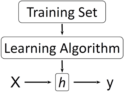The hypothesis here is nothing but a linear equation which resembles the equation of a line. Our hypothesis function has the general form: hθ(x)=θ0+θ1x where θ1 is the slope of the line and θ0 is the constant.

We can see that it can be more or less fit to a straight line if we plot the training set.

What are the Errors of Prediction?

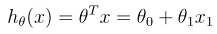
The black diagonal line in the figure is the regression line and consists of the predicted score on Y for each possible value of X. The vertical lines from the points to the regression line represent the errors of prediction. As you can see, the red point is very near the regression line; its error of prediction is small. By contrast, the yellow point is much higher than the regression line and therefore its error of prediction is large.

What is the Least Squares Method?

Linear regression models are often fitted using the least squares approach. Statisticians call this method for finding the best-fitting line as: simple linear regression analysis using the least squares method. The least squares approach can also be used to fit models that are not linear.

What is the Cost Function J?

The cost function is what we want to minimize. In this example our cost function will be the sum of squared errors over our data or training set. The “distance” is the vertical distance between the predicted y and the observed y. This is also known as the residual. The objective of linear regression is to minimize this cost function.

Gradient Descent Explained

Gradient descent is one of those awesome algorithms that offers an incredibly simple way to minimize a function iteratively and a new perspectives for solving problems. Gradient descent is a method for finding the minimum of a function of multiple variables. So you can use gradient descent to minimize our cost function.

At a theoretical level, gradient descent is an algorithm that minimizes functions. Given a function defined by a set of parameters, gradient descent starts with an initial set of parameter values and iteratively moves toward a set of parameter values that minimize the function. This iterative minimization is achieved using calculus, taking steps in the negative direction of the function gradient.

It’s sometimes difficult to see how this mathematical explanation translates into a practical setting, so it’s helpful to look at an example. The canonical example when explaining gradient descent is, by the way, linear regression.

What is the Gradient Descent Intuition?

The gradient of a function is a vector which points towards the direction of maximum increase. Consequently, in order to minimize a function, we just need to take the gradient, look where it’s pointing, and head the other direction.

The derivative is the slope as shown using a red line.

Case (a): A positive derivative/slope which will allow the new theta1 to move to left (Smaller) to converge.

Case (b): A negative derivative/slope which will allow the new theta1 to move to right (Bigger) to converge.

How to Compute the cost J(θ)?

Lets define a cost function that measures how good a given prediction line is. This function will take in a pair and return an error value based on how well the line fits our data. We will iterate through each point in our data set and sum the square distances between each point’s y value and the candidate line’s y value to compute this error for a given line. It’s conventional to square this distance to make our function differentiable and to ensure that the result is always positive.

where the hypothesis h θ (x) is given by the linear model:

In this part, you will fit the linear regression parameters θ to our dataset using gradient descent. The parameter alpha is a learning rate usually just some small number that you can tune to adjust how fast your algorithm runs. Thus, gradient descent can be succinctly described in just a few steps:

1. Choose a random starting point for your variables.

2. Take the gradient of your cost function at your location.

3. Move your location in the opposite direction from where your gradient points, by taking your gradient ∇g, and subtract α∇g from your variables, where α is the learning rate.

4. Repeat steps 2 and 3 until you’re close to the minimum.

What are Advantages and Limitations?

So far, we have only been able to examine the relationship between two variables. The main advantage of linear regression is its simplicity, scientific acceptance, interpretability, and availability. Linear regression is the first method to use for many problems. This technique is useful when trying to account for potential confounding factors in observations. Linear regression implements a model that shows optimal results when relationships between the independent variables and the dependent variable are almost linear. Linear regression is widely available in software packages and business intelligence tools.

Linear regression main limitation is that in many real-world scenarios it does not correspond linear models. Linear regression is often inappropriately used to model non-linear relationships. Linear regression is limited to predicting numeric output. It is also difficult or impossible to generate good results with linear regression in these cases.

Machine Learning & the Best Ever Investment

Brain” by TZA is licensed under CC BY 2.0 on Flickr

Smart people are often searching for the best destination of their resources. They know the value of time. They take time to dig into the details and evaluate the consequences of each of their actions. They also know the value of generosity and generously share the findings along the way. This is the case of the Bill Gates.

In his recent post “Setting Targets to Save Lives” he exposed what seems to be a unique and unbeatable investment:

“Can you beat a nine-fold return on investment, saving more than 61 million children and 3 million mothers, and preventing 21 million deaths from AIDS and 10 million from TB? Frankly, I doubt it. But if you can, I would love to see your plan.”

This amazing 900% ROI is based on a the “Global Health 2035” finding that over the period 2015–2035, the economic benefits of Global Health convergence would exceed costs by a factor of about 9 in low-income countries and around 20 in lower-middle income countries. This benefit cost ratio makes the investment extremely attractive.

In the same post Gates also mentions the role of research on health topics in this investment scenario:

“The report also found that in the near term, the 34 richest nations will need to expand their efforts, especially funding for research on new vaccines and other lifesaving tools.”

As a student of the most popular course at Stanford I have been on top of the impact Machine Learning has created in the field of Health-care. Machine Learning has been successfully used not only to support the development of new vaccines but to develop software applications that promote healthy behaviors in consumers, support care givers, personalize medical treatments, improve the understanding of emotional states, improve stem cell therapies, predicting how viruses will change over time within specific individuals and much more.

But, what is Machine Learning?

Machine learning is the science of collecting and analyzing data and turning it into predictions, encapsulated knowledge, or actions. Machine learning focuses on the development of computer programs that can teach themselves to grow and change when exposed to new data. Traditional machine learning techniques, including classic neural networks, need to be supervised by humans so they can learn. Deep learning is a very special subcategory of machine learning and an emerging topic in artificial intelligence. Deep learning is an attempt to have the system learn on its own, without human intervention.

The Machine Learning Momentum

The commercial success and widespread use of machine learning has attracted the attention of big companies and investors worldwide. They are hiring top talents: My professor at Coursera and Google’s deep-learning visionary Andrew Ng was recently snatched by Baidu as its chief scientist. NYU Professor Yann LeCun, a respected pioneer in artificial intelligence, was recently hired by Facebook .

In the field of acquisitions, Google reportedly paid $500 million for the acquisition of DeepMind, a start-up based in London that had one of the biggest concentrations of researchers anywhere, working on deep learning. Twitter alone acquired Madbits, a deep learning and dynamic computing startup and Whetlab, a Cambridge-based machine learning startup. IBM acquired AlchemyAPI, a deep learning startup to enhance Watson’s Deep Learning Capabilities. Microsoft bought Revolution Analyticsfor deeper data analysis. Yahoo acquired LookFlow to work on Flickr and ‘Deep Learning’.

The Machine Learning Talent Shortage

The study Big data: The next frontier for innovation, competition, and productivity by the McKinsey Global Institute (MGI) projects there will be approximately 140,000 to 190,000 unfilled positions of data analytics experts in the U.S. by 2018. This other source predicts a 50 to 60 percent gap between the supply and demand of people with deep analytical talent. These “data geeks” have advanced training in statistics or machine learning as well as the ability to analyze large data sets.
In his article What’s Causing The IT Talent Shortage? Alex Espenson, a recently retired business owner turned consultant, mentions Machine Learning as one of the skills in high demand:

 “Organizations are looking for professionals with very specific specialties, like data science, cloud computing and machine learning. The problem is, there just aren’t enough people with these skills.”

Solutions

The “Tools” Approach

Business intelligence and analytics providers are responding to the continuing shortage of machine learning experts by offering machine learning know how as a cloud service. The “Machine Learning as a Service” (MLaaS) solution is one of them, launched about the same time as the Google Prediction API and BigML.

There was a similar talent shortage some years ago with website development. Web Content Management Systems such as Joomla was used to resolve most of the needs. Note that you still need expert web developers for the most specialized use cases.

I have the feeling that the same situation is happening in Machine Learning right now. Solutions implemented as tools for domain experts as the above mentioned MlaaS, BigML and Google Prediction API are just the current way around the talent shortage. However, this will meet only the more generic needs like those related to extracting knowledge from web server logs.

The “People” Approach

Alternatively, others are turning to Outsource Analytics in different counties worldwide. Latin America is already acting upon these needs.

Governments are encouraging companies to boost their own human capital by providing on-the-job training. For example, the government agency Uruguay XXI’s “finishing schools” initiative offers subsidies to export-oriented companies to train staff in specific skills, such as English, and help them to master new technologies. Early this year Chile Inaugurates Latin America’s Largest Robotics Show that exhibits concrete technological solutions for present as well as future challenges.

Since 2004 the University of Buenos Aires offers a Master in Data Mining and Knowledge Discovery. It is the first Latin American university to offer a program in this increasingly popular specialty to train professionals to discover and detect patterns, relationships and make models from huge data sets. In Peru, Carlos Rodriguez-Pastor has established 23 Innova schools, serving 13,500 students, where teachers’ knowledge and skills are continuously updated. Other countries are also providingsimilar programs.

The industry is also moving along this technology trend. For example, robots weld carsat the Ford Motor Company’s Sao Bernardo do Campo facility and moves chassis along the assembly line in Aguascalientes, Mexico. One of the most interesting startups in São Paulo is Loggi, which focuses on urban deliveries. Loggi’s founder Fabien Mendez likes to point out that the company’s core competency is to apply machine learning and mathematics to logistics’ optimization. In his own words:

“There are five algorithmic dimensions to combine: dispatching, routing, volumetric placement, scheduling and bundling,”

Latin American businesses in the Brazilian state of São Paulo have research contracts with leading public universities. Such links have helped to lift São Paulo’s R&D spending to 1.6% of GDP – higher than that of Spain or Italy.

Now that Latin America is creating the talents with the skills to extract value out of huge data sets, it may be a good time to consider the region as a potential target of our talent search. It may be now the right time to consider nearshore engineering services companies in Latin America if you’re still in need of machine learning experts. We are actively moving forward with the technology and have years of experience and the ability to quickly catch up with this and any required domain expertise.